Thanks to the many online explanations of the Y combinator in lambda calculus (LC), I think I'm finally getting the hang of it, though the critical step was trying it myself and suffering through the pitfalls. Unfortunately my education screwed me on the conceptual front, never introducing me to wizard book ideas, and I've spent my life in an imperative programming cave. There's a barrier of terminology too. You don't define functions, you define abstractions. You don't call functions, you apply them. You don't evaluate a function, you beta reduce. No function takes multiple parameters, they take one parameter and return a function that deals with the remainder, a concept called currying.
I especially liked Todd Brown's analogy that LC is like functional programming's (FP) creation myth, and as an FP adherent, he was due to perform the pilgrimage to FP's roots. I'm not an FP devotee yet, though I am intrigued, but I performed the same pilgrimage and it has been well worth it! Prior, when I imagined the most abstract device capturing the essence of computation, my mind had a single path that ended with symbols on tapes and a commanding state machine. Now there's a whole alternative universe where only functions float about, and by positioning these functions into arcane arrangements, you are able to represent and compute anything.
It's not a mere sightseeing tour either. I've grown a bit fond of the idea, and imagine it as "curvy" or "fluid" and possibly a more natural conceptual foundation for computation than the cold mechanical machinery of a Turing machine. Maybe it's that fancy swoosh down the right side of that Greek lambda symbol. Related, Tomas Petricek has a cool blog post Would aliens understand lambda calculus?.
Studying LC leads to to what seems like its crown jewel idea: the Y combinator. There are an abundance of angles by which people online try to explain the Y combinator, but it was still very slow for me to absorb. I found that they fall into two approaches:
I'll repeat the explanations below, paraphrased in a way that both reminds me in the future when I look back to these notes, but also in a way I wish I had found when searching for an explanation.
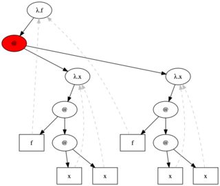
The Y combinator is the lambda term \f[(\x[(f (x x))] \x[(f (x x))])] which looks like this in graph form:
The red highlights the application that would occur next in normal reduction strategy. Watch what happens if you provide it no argument, and beta reduce:
\f[(\x[(f (x x))] \x[(f (x x))])]
\f[(f (\x[(f (x x))] \x[(f (x x))]))]
\f[(f (f (\x[(f (x x))] \x[(f (x x))])))]
\f[(f (f (f (\x[(f (x x))] \x[(f (x x))]))))]
...
You can see that it repeatedly applys parameter f to itself. In graph form:
By letting symbol Y represent its full expression, we get a more compact representation:
Y
(f Y)
(f (f Y))
(f (f (f Y)))
...
Or:
Y         @          @           @          ...
         / \        / \         / \
        f   Y      f   @       f   @
                      / \         / \
                     f   Y       f   @
                                    / \
                                   f   Y
Why doesn't thisresult in infinite regress? Actually it does, when no argument is provided to Y, but Y is a higher order function, and thus expects an abstraction f. Since the leftmost, outermost is evaluated first, f gets to decide whether to use a further expansion of Y (recursion) or discard it (base case).
Let's pretend f is the triangle numbers function, written recursively:
def triangle(n):
    if n == 0: return 0
    return n + triangle(n-1)
But in lambda calculus, all functions are anonymous, so we can't make use of that name "triangle" to recur. Get it into form:
def triangle(f, n):
    if n == 0: return lambda n: 0
    return lambda n: n+f(n-1)
Note the first parameter is discarded for the base case, which will discard the next expansion of Y.
Here's how computation starts for ((Y triangle) 2), the first reduction happens within the combinator:
      @             @
     / \           / \
 -> @   2      -> @   2
   / \           / \
  Y  tri       tri  @
                   / \
                  Y  tri
Now tri is in position for reduction. It evaluates its arguments f and 2 and since 2 is not the base case, the next call to Y remains:
     @          -> @            "+"
    / \           / \           / \
-> @   2         λ   2         2   @
  / \            |                / \
tri  @           @            -> @   1
    / \         / \             / \
   Y  tri      Y  tri          Y  tri
So here we go, Y expands again:
  "+"            "+"            "+"           "+"
  / \            / \            / \           / \
 2   @          2   @          2   @         2  "+"
    / \            / \            / \           / \
-> @   1       -> @   1       -> λ   1         1   @
  / \            / \             |                / \
 Y  tri        tri  @            @            -> @   0
                   / \          / \             / \
                  Y  tri       Y  tri          Y  tri
Last time:
  "+"           "+"            "+"             "+"
  / \           / \            / \             / \
 2  "+"        2  "+"         2  "+"          2  "+"
    / \           / \            / \             / \
   1   @         1   @          1   @           1   0
      / \           / \            / \
  -> @   0      -> @   0       -> λ   0
    / \           / \             |
   Y  tri       tri  @            @
                    / \          / \
                   Y  tri       Y  tri
The base case happens when ((triangle (Y triangle)) 0) because the outermost triangle is evaluated first, taking the (Y triangle) parameter then the 0 parameter and discarding the former, since it's defined to return 0 when n==0.
So that's it. Y is just a lambda term. It gains the badge of "combinator" by having no free variables. And it applies the argument to an application of Y applied to its argument.
The task of solving equations can be transferred to the task of finding fixed points. Suppose you want to solve x^2 + 3x + 2 = 0. That can be manipulated to a recursive definition x = (x^2 + 2)/3 and we can take the right hand side to construct a generating function (GF) f(x) = (x^2 + 2)/3 whose fixed points are x=1 and x=2, the solutions to the original. The book Design Concepts in Programming Languages states compactly:
A solution to a recursive definition is a fixed point of its associated generating function.
If x is a fixed point of f(x) then it's also a fixed point of the composition f(f(x)) and f(f(f(x))) and so on. Here they are graphed:
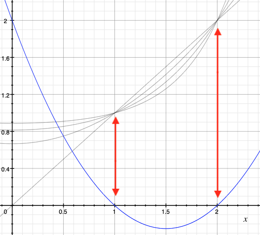
The blue curve is the original quadratic with visible roots at x=1 and x=2 and the three gray curves all intersect at the fixed points.
In x = (x**x + 2)/3 the solution space of x is the domain of real numbers. Solutions are also fixed points of the generating function f(x) = (x**x)+2: 1 and 2.
In f = lambda f,n: 0 if n=0 else 2+f(n-1) the solution space of f is the domain of functions. Solutions are also fixed points of generating function lambda n: 0 if n=0 else 2+f(n-1): lambda n: 2*n.
That's the trick. You don't explicitly construct a recursive function like you would in an imperative language. You instead construct a generator function that's a higher order function (HOF) whose fixed point is the function with the desired behavior, and apply the fixed point operator Y to obtain it.
It's easy to get confused since the HOF looks very much like the desired function.
Suppose you wanted a doubling function, something like:
def double(n):
  if n==0: return n
  return 2 + double(n-1)
This calls itself, double(n-1) which doesn't exist in LC. The higher order function is:
def double_HOF(f):
  return lambda n: return 0 if n==0 else 2*n + f(n-1)
It has type (N -> N) -> (N -> N). It takes a function that operates on reals, and returns a function that operates on reals. Don't let it get too abstract! You could write an input/output table, leaving the function parameter f variable and choosing sequential concrete naturals for n:
  f(n)    n     result
  ----    -     --------
  f(0)    0     0
  f(1)    1     2 + f(0)
  f(2)    2     2 + f(1)
  f(3)    3     2 + f(2)
  ...
So what function f is there such that f(1) = 2 + f(0) and f(2) = 2 + f(1) and f(3) = 2 + f(2) and so on? It's the same as solving f = double_HOF(f) for some f with type (N -> N). It's the same as finding the fixed point. The solution is returned by fix(double_HOF) which is double:
  f(n)             n    result
  ----           -    ------
  double(0)=0      0    0
  double(1)=2      1    2 + double(0) = 2
  double(2)=4      2    2 + double(1) = 2 + 2 = 4
  double(3)=6      3    2 + double(2) = 2 + 4 = 6
  ...
Note the actual lambda term returned from (fix double_HOF) would not be the as the lambda terms from a direct translation of double. You couldn't translate double, since
def fact(n):
  if n==0: return 1
  return n*fact(n-1)
Our generating function, or higher order function is:
def fact_HOF(f):
  return lambda n: return 1 if n==0 else n*f(n-1)
It takes functions (N -> N) and returns functions (N -> N). Using lambda notation now, for any input f it returns a new f = λn.((* n) (f ((- n) 1))).
Let's now send some n values to the f on the left hand side (lhs) and right hand side (rhs).
n     lhs(n)    rhs(n)
-     ------    ------
0     (f 0)     1
1     (f 1)     ((* 1) (f ((- 1) 1)))
2     (f 2)     ((* 2) (f ((- 2) 1)))
3     (f 3)     ((* 3) (f ((- 3) 1)))
...
Since we have the setup f = fact_HOF(f) we can solve for the fixed point f with (fix fact_HOF). But what function f fits the definition, making the lhs and rhs equal? Factorial of course. Let's test it:
n     lhs(n)         rhs(n)
-     ------         ------
0     (fact 0) = 1   1
1     (fact 1) = 1   ((* 1) (fact ((- 1) 1))) = ((* 1) (fact 0)) = ((* 1) 1) = 1
2     (fact 2) = 2   ((* 2) (fact ((- 2) 1))) = ((* 2) (fact 1)) = ((* 2) 1) = 2
3     (fact 3) = 6   ((* 3) (fact ((- 3) 1))) = ((* 3) (fact 2)) = ((* 3) 2) = 6
...